Voices, under the microscope.

Dudley's VODER (Voice Operation Demonstrator) is the first documented machine to produce intelligible continuous speech from a non-speech source. There was no magnetic tape playback, no database of recordings, no computer. The machine had two sound sources — a buzzing relaxation oscillator for voiced sounds, a gas-discharge tube for unvoiced hiss — selected by a foot pedal. Ten bandpass filter keys on the operator's right hand gave fingertip control over ten vocal-tract resonances from roughly 500 Hz to 7.5 kHz. A wrist bar modulated pitch. Three extra keys produced the burst-release timings for stops like /t/, /p/, /k/.

It took the bank of operators — a team of women hand-picked from Bell's phone-service division — roughly a year of daily practice to play a sentence cleanly. A single demonstration required about the same rehearsal as a concerto. The result: a recognizable, somewhat ghostly, clearly human voice under manual control. Audio and film from the World's Fair survive; modern acousticians still point to VODER as the first proof that the vocal tract is, mathematically speaking, a filter bank.

The crucial move was conceptual. Dudley separated what drives the vocal folds from what the throat and mouth do to that source. That separation, and a bank of bandpass filters to shape the result, turned out to be universal enough that every later system is either a direct descendant or a refutation of it.

The Sound Spectrograph is the ancestor of every figure on this page. Input speech was recorded onto a magnetic tape loop, typically about 2.4 seconds long. A rotating drum dragged the loop past a playback head over and over. In parallel, a single variable-frequency bandpass filter swept slowly from 0 to about 4 kHz through heterodyning. Each time the filter's center frequency completed another scan, an electric stylus burned a horizontal stripe onto sensitized paper wound around a synchronized drum. Darker stripes meant the filter had found more energy in that band.

The output was a rectangle. Time ran left to right, frequency ran bottom to top, darkness encoded amplitude. Linguists immediately saw that formants — the resonances Dudley's VODER filters had imposed manually — appeared as dark horizontal bands. The spectrograph gave the field its shared vocabulary: F1, F2, F3 are named after the tracks on a 1950 spectrogram. Dennis Klatt would later use spectrograms as targets when tuning his synthesizer rules. The training data of every modern TTS model is, structurally, just a digital spectrograph running on millions of utterances.

The machine is beautiful to look at. It's also incredibly slow: each 2.4-second clip takes about four minutes to render, because the filter has to sweep mechanically. The arrival of the FFT (Cooley & Tukey, 1965) made the process real-time on general-purpose computers and killed the physical spectrograph as a laboratory tool — but the visual it invented has never been replaced.

Linear prediction coding (LPC) formalized the intuition VODER made with wires. The claim: each speech sample can be predicted as a linear combination of the previous p samples plus a residual. The residual carries the excitation (a buzz when voiced, a hiss when not), and the predictor coefficients describe the vocal tract as an all-pole IIR filter. Ten to sixteen coefficients per 20-millisecond frame reproduce speech that is recognizably human.

Mathematically, the poles of H(z) = 1 / A(z) land near the formants. Fit the coefficients via the Levinson–Durbin recursion (linear time in p), store them as line spectral pairs (LSP) for numerical robustness, transmit at a few kilobits per second, and you have the backbone of every low-bitrate speech codec of the 1980s and 1990s. The GSM mobile standard's RPE-LTP codec is a direct child of LPC. So is the DoD 2.4 kbit/s LPC-10 military codec. Klatt's formant synthesizer used LPC as a tuning aid.

For TTS, LPC didn't produce natural speech on its own. The residual is hard to predict from text. But the source–filter abstraction — excitation at one end, spectral envelope in the middle, radiation at the output — is the frame that every later vocoder (from Klatt's to WaveNet's) implicitly or explicitly inherits.

Klatt's formant synthesizer was the final triumph of the rule-based era. A voicing source, an aspiration source, and a frication source are combined in two parallel branches: a cascade of up to five digital resonators for voiced speech (each formant feeds the next), and a bank of parallel resonators with per-formant amplitudes for fricatives, affricates, and nasals. About 60 parameters, updated every 5 ms. That is enough to say anything.

The genius was in the rule set. Klatt wrote, by hand, the expected formant trajectories and voicing patterns for every English phoneme in every context. Tens of thousands of rules. The result, commercialized as DECtalk, became the voice that Stephen Hawking used for decades (Klatt's voice model PBJOHN remained on Hawking's speech computer until his death — he explicitly refused upgrades because he had come to identify with it).

What killed Klatt synthesis was naturalness. The speech was perfectly intelligible — more intelligible than most modern TTS for technical terms, numbers, and rare words — but it sounded like a robot. The hand-written rules couldn't capture the fine-grained prosody that makes a voice sound alive. Unit-selection TTS of the 1990s kept the intelligibility and added the naturalness, at the cost of a much larger footprint.

Concatenative synthesis replaced rules with recordings. A voice actor sits in a studio for a week and reads a couple thousand carefully chosen sentences. The audio is phonetically segmented, catalogued by linguistic context, and stored. At synthesis time, the system picks diphone or phone units from the database using Viterbi search over two costs: a target cost (how well a candidate matches the target context: preceding phoneme, following phoneme, stress, position in phrase) and a join cost (how spectrally continuous two consecutive candidates are at their boundary).

Inside the recorded domain, the result is astonishing. AT&T's Natural Voices and early Loquendo demos are still hard to distinguish from human speech if you only listen to short, prosaic utterances. The data model is the speaker, so pronunciation is correct by construction. Emotional range is limited by what the voice actor recorded; out-of-domain words (rare names, code-switched words, new brand terms) cause audible seams because the Viterbi search has to force-fit units that don't quite match.

The approach's unforgivable weakness is scale. Every new voice requires a new multi-day recording. Every new style (cheerful, solemn, whispered) either needs its own recorded set or shows audible mismatch. Databases grew to gigabytes — unshippable to mobile. A generation of practitioners wanted to go back to parametric synthesis, but with machine-learned parameters instead of Klatt's hand rules.

HMM-based TTS returned to the parametric path with a statistical twist. Every phoneme in every context becomes a left-to-right hidden Markov model. Each state emits three parameter streams: a spectral envelope (mel cepstrum + deltas), a pitch contour (log F0 modeled with multi-space distributions that handle voiced/unvoiced regions), and a duration (modeled with a hidden semi-Markov extension so states can stay as long as needed). Training sees labeled speech, estimates Gaussian emissions for each state, then clusters states across contexts using decision trees so rare contexts still get sensible parameters.

At synthesis, the system picks a sequence of states from the decision trees using the target labels, generates parameters, and runs them through a vocoder — typically STRAIGHT or later WORLD. The flexibility was revolutionary. Want to make the voice happier? Retrain only on happy speech. Want a new speaker with an hour of audio? Adapt the existing model with MLLR. Want a new language? Just relabel. The downside was that everything sounded slightly muffled: the max-likelihood trajectory of a Gaussian HMM is inherently over-smoothed. HMM-TTS never reached unit-selection's peak naturalness, but it reached good-enough naturalness everywhere instead of excellent naturalness in-domain.

HTS is the direct ancestor of every modern TTS pipeline. Its labels became FastSpeech's phoneme-level features. Its three-stream modeling became FastPitch's separate pitch head. Its decision tree clusters foreshadowed speaker embeddings. The ideas are load-bearing even where the name is forgotten.

WaveNet modeled raw audio directly: one sample at a time, conditioned on every previous sample in the sequence, with categorical outputs over 256 mu-law-quantized levels. The architectural contribution was the dilated causal convolution: by doubling the dilation rate each layer, a 30-layer stack reaches a receptive field of tens of thousands of samples (seconds of audio) while remaining a feed-forward convolution during training. The network was conditioned on linguistic features — essentially the outputs of a classical TTS front-end — that told it which phoneme, with which pitch, for which speaker.

Naturalness jumped to within a single MOS point of human speech, beating every concatenative system on the same voice. The cost was brutal: because the model is autoregressive at the sample level, inference at 16 kHz requires running the stack 16,000 times per second. On the original GPU implementations a minute of audio took hours. Parallel WaveNet (Oord et al. 2017) distilled the autoregressive model into an inverse-autoregressive flow that generates audio in a single parallel pass, but the distillation was fragile and the student model rarely matched the teacher.

WaveNet did two things that stuck. It proved that a neural vocoder could close the gap between statistical parametric speech and concatenative speech. And its stacked dilated convolutions became the backbone block for essentially every fast follow-up — Parallel WaveGAN, MelGAN, HiFi-GAN — even when they discarded the autoregressive frame.

Tacotron was the first successful attempt at “put text in, get audio out, no linguistic front-end” — a single neural network trained end-to-end. An encoder (a CBHG block: 1D convs, highway layers, bidirectional GRU) consumed character embeddings and produced a per-character hidden state. An attention module aligned these hidden states to the target audio timeline. A decoder (an autoregressive LSTM) emitted mel-spectrogram frames one at a time, each conditioned on the previous frame and the attention-weighted encoder states. For the original paper the mel was turned back into audio via Griffin-Lim, the classical non-neural phase-recovery algorithm.

The elegance was the intermediate representation. Text→mel is a manageable supervised learning problem (aligned data at tens of milliseconds, not tens of microseconds). Mel→audio is a separable vocoder problem (trainable with a different loss on a different dataset, including data without paired text). Splitting the problem this way turned out to be a strictly better engineering choice than WaveNet's sample-level modeling for everything except the highest-end server deployments.

Tacotron 2 (2018) swapped the CBHG encoder for stacked convolutional and LSTM layers, used a location-sensitive attention to stabilize alignment on long utterances, and replaced Griffin-Lim with a WaveNet vocoder conditioned on the predicted mel. The result was mean-opinion-score parity with human recordings on short, neutral utterances. This is the point at which “neural TTS” stopped being a research curiosity and became a product surface.

FastSpeech replaced Tacotron's autoregressive decoder with a parallel one. The trick was an explicit duration predictor: for each phoneme, predict how many mel frames it should span, then use a length regulator to simply repeat the phoneme embedding that many times. The expanded sequence is decoded by a stack of self-attention + convolution blocks in parallel — no recurrence, no attention to encoder states at inference. FastSpeech 2 added explicit pitch and energy predictors, drawing on the HMM-TTS lineage.

HiFi-GAN solved the vocoder speed problem. Where WaveNet generated one sample at a time and Parallel WaveGAN used a complex flow-based training recipe, HiFi-GAN was a straight convolutional generator trained with two classes of discriminator: a multi-period discriminator (MPD) that looks at the signal rearranged into 2D patches with various period lengths (catching periodic artifacts), and a multi-scale discriminator (MSD) that looks at the signal at full rate, half rate, quarter rate (catching scale-specific distortion). Plus a mel-L1 reconstruction loss. Adversarial feature matching for stability.

Combined, FastSpeech + HiFi-GAN could generate 22-kHz speech at dozens of times real-time on a single consumer GPU, with quality indistinguishable from Tacotron 2 on most listening tests. This is the point at which the “ship a custom TTS” curve crossed below a hundred GPU-hours.

VITS collapsed the FastSpeech + HiFi-GAN pipeline into one network. A posterior encoder reads the target spectrogram and emits a latent z. A HiFi-GAN-style decoder reconstructs the waveform from z. A prior over z is learned from the text side via a normalizing flow that transforms a standard Gaussian conditioned on the encoded text. The ELBO ties the two — reconstructing the target waveform and matching the flow-transformed Gaussian at training time. Monotonic Alignment Search (MAS) replaces attention with a dynamic-programming alignment between text and spectrogram frames.

The effect: one optimizer, one training loop, one set of weights. Quality matches or exceeds two-stage FastSpeech + HiFi-GAN while avoiding the mismatch that accumulates when you train text→mel and mel→audio independently. The decoder discriminators (inherited from HiFi-GAN) keep the waveform sharp. The flow prior keeps the latent space multi-modal so the model can express prosodic variation.

VITS was the first open model where “paper-quality end-to-end TTS” was within a few days of training reach for a hobbyist with a single GPU. Its open-source implementation drove most of the community TTS ecosystem (Coqui-AI, SambertHifiGan, StyleTTS) through 2022 and 2023.

StyleTTS2 introduced two ideas. First, an entire utterance's style — speaker identity, emotional tone, recording-room texture — is compressed into a single style vector s. This vector is used to modulate every LayerNorm in the acoustic decoder through style-adaptive layer norm (SALN): the affine parameters of LN are themselves predicted from s. You get rich conditioning without adding layers to the decoder trunk.

Second, the style vector is not predicted directly. It is produced by a tiny diffusion model conditioned on the text's semantic embedding. At inference, you run 32 denoising steps on a Gaussian latent and get a style vector. This is the only diffusion step in the pipeline — the audio itself is decoded with a fast iSTFT-based vocoder. The result is diffusion-quality expressivity without diffusion-cost inference.

StyleTTS2 was among the last open architectures before flow matching became the community default for new systems. Its quality on the LJSpeech benchmark was competitive with much larger closed models at ∼150M parameters. Kokoro-82M — the model powering every audio clip on this page — is a smaller, curated training of the same architecture, with the style diffusion frozen into a lookup of pre-computed per-voice style vectors so inference runs on CPU.

Flow matching is the formulation that superseded DDPM-style diffusion for audio in 2024. Instead of learning the score of a noising process, flow matching directly learns a vector field that transports a simple distribution (pure noise) to the data distribution along straight or near-straight paths. Training loss is an MSE between the predicted vector field and a hand-chosen ground-truth field derived from a noise-to-data coupling. Inference is ODE integration — typically 4 to 16 Euler steps, an order of magnitude fewer than diffusion, with equal or better quality.

F5-TTS (Flow matching for Speech synthesis, with diffusion Transformer) brought this approach to open-source TTS. Unlike VITS or StyleTTS2, F5-TTS is a one-stage system that predicts a mel spectrogram directly via flow matching on a transformer trunk. It matches or exceeds commercial API TTS on standard MOS tests while being fully reproducible on public data. It is also the first fully permissively licensed (MIT) model where the community can legitimately finetune and redistribute derivatives.

MaskGCT and NaturalSpeech 3 take a different route: the target is a neural audio codec (EnCodec, SoundStream, DAC), which turns audio into a sequence of discrete tokens. The TTS model masks tokens and is trained to predict them from context, like BERT but generative. At inference, the model iteratively unmasks tokens in order of confidence, doing parallel prediction within each step. These discrete-token systems are currently the quality leaders on zero-shot voice cloning benchmarks.

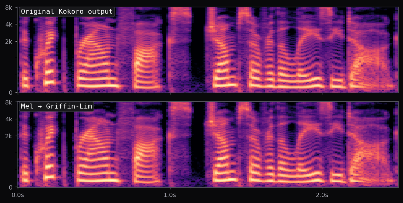
Kokoro-82M is a distillation and community-curated training of the StyleTTS2 architecture at roughly 82M parameters — about half the size of the reference StyleTTS2 release. The style diffusion step is pre-computed per voice and stored as a fixed embedding; inference is therefore a single forward pass through the acoustic model plus an iSTFTNet vocoder. End-to-end latency on a modern laptop CPU is under 400 ms for a full sentence.

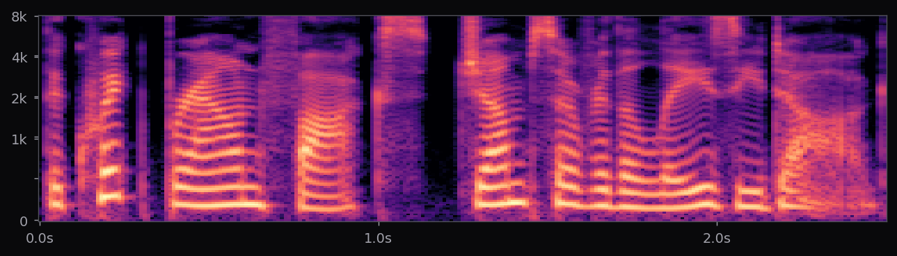
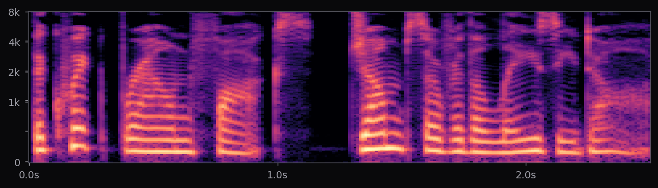
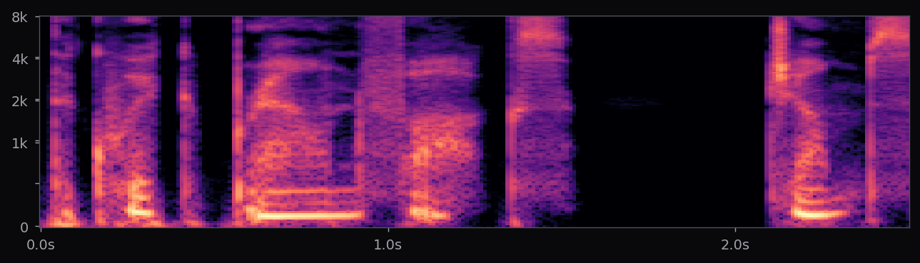
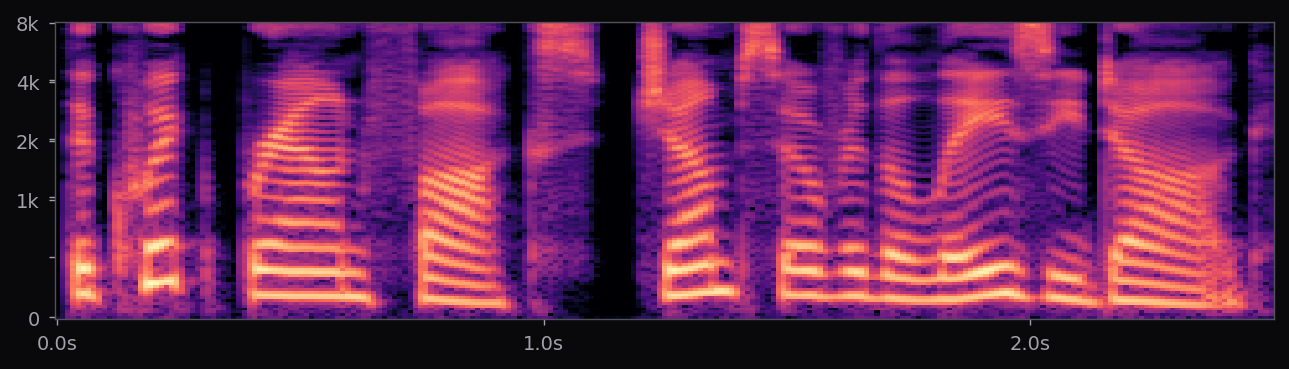
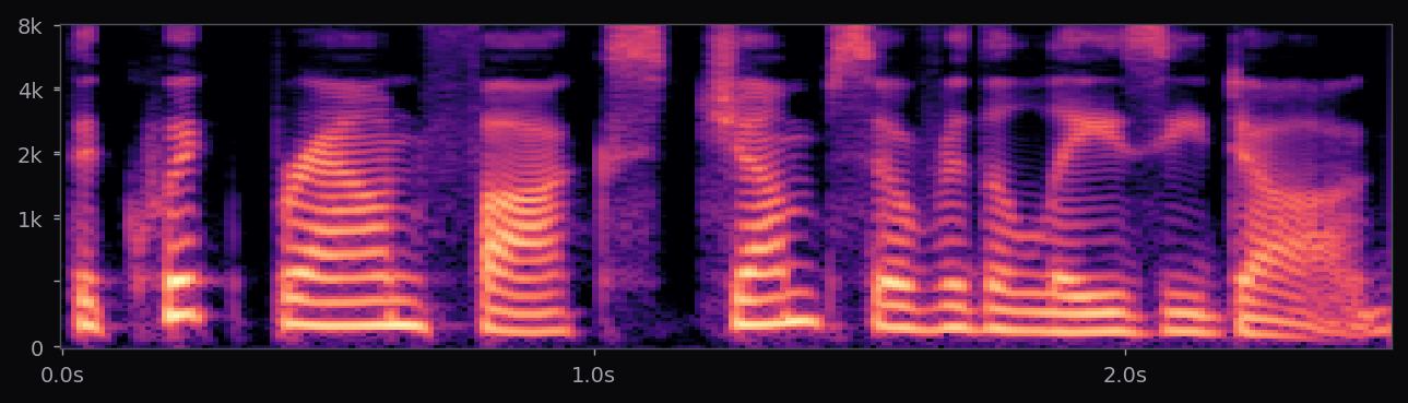
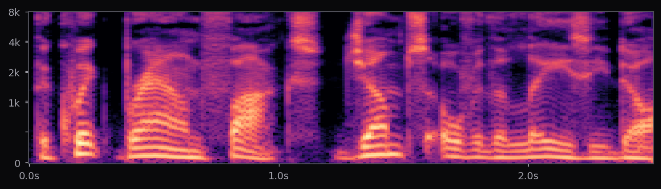
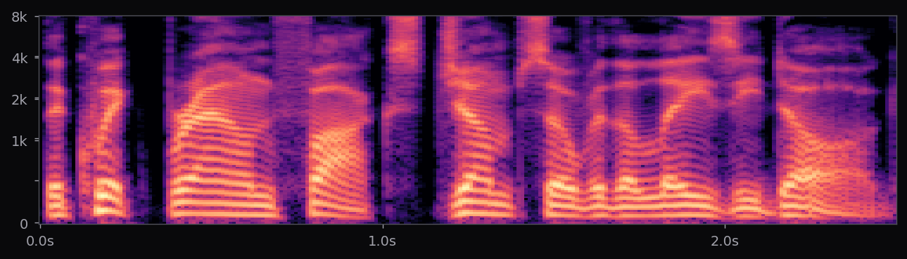
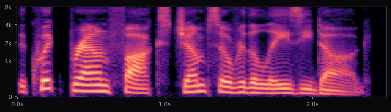
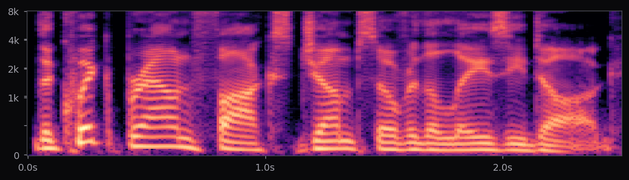
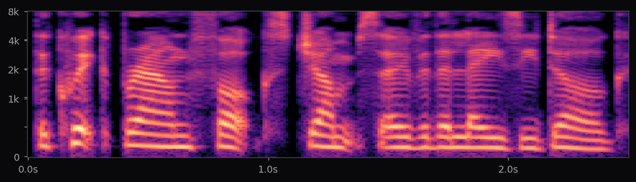
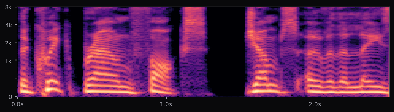
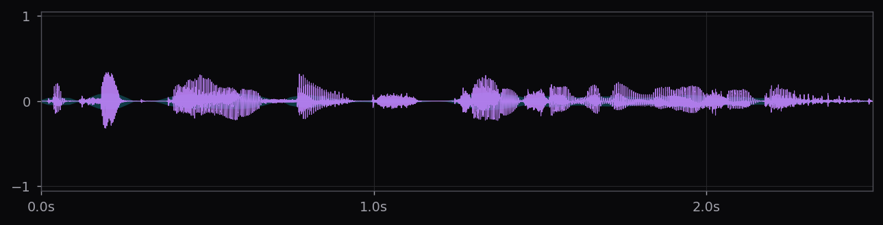
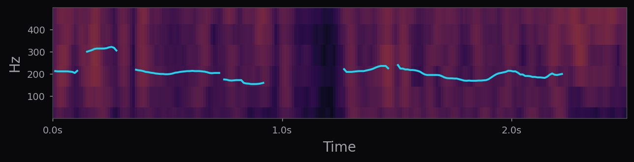
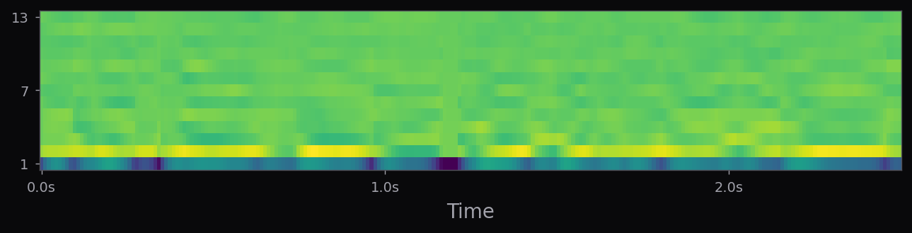
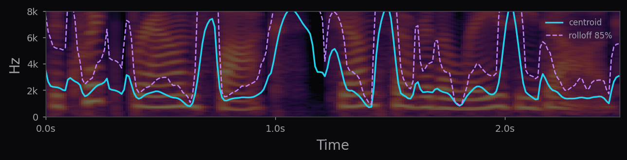
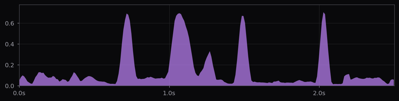
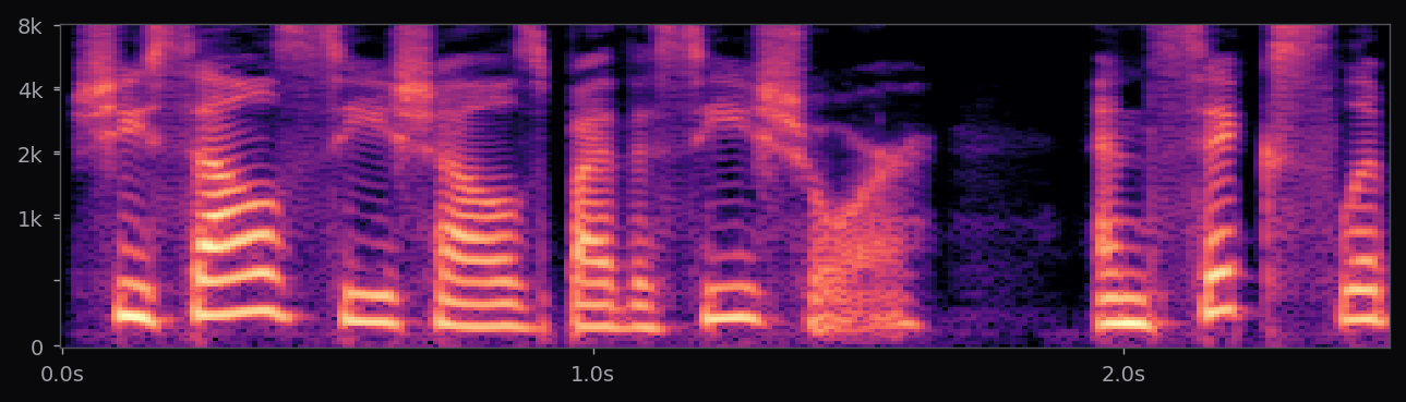
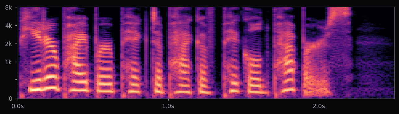
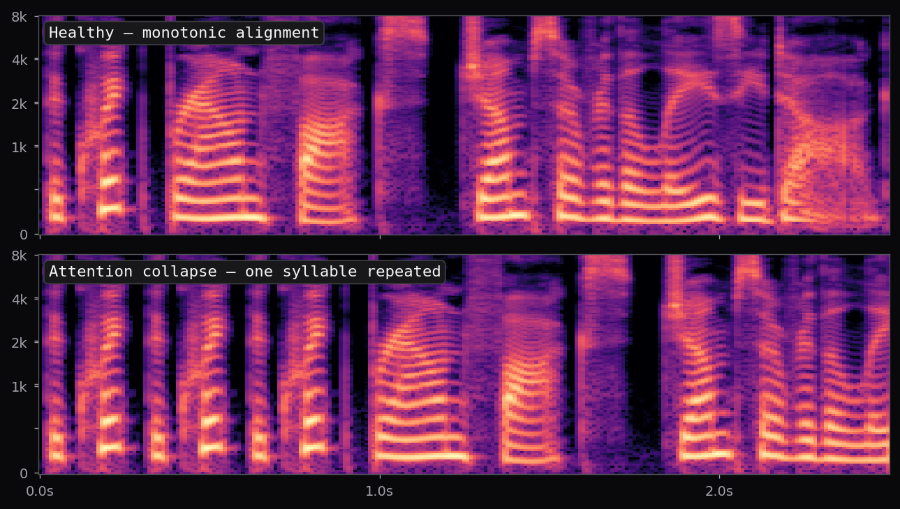
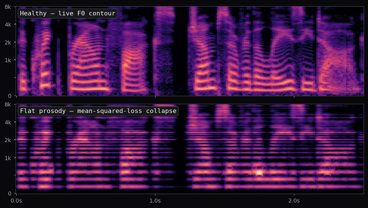
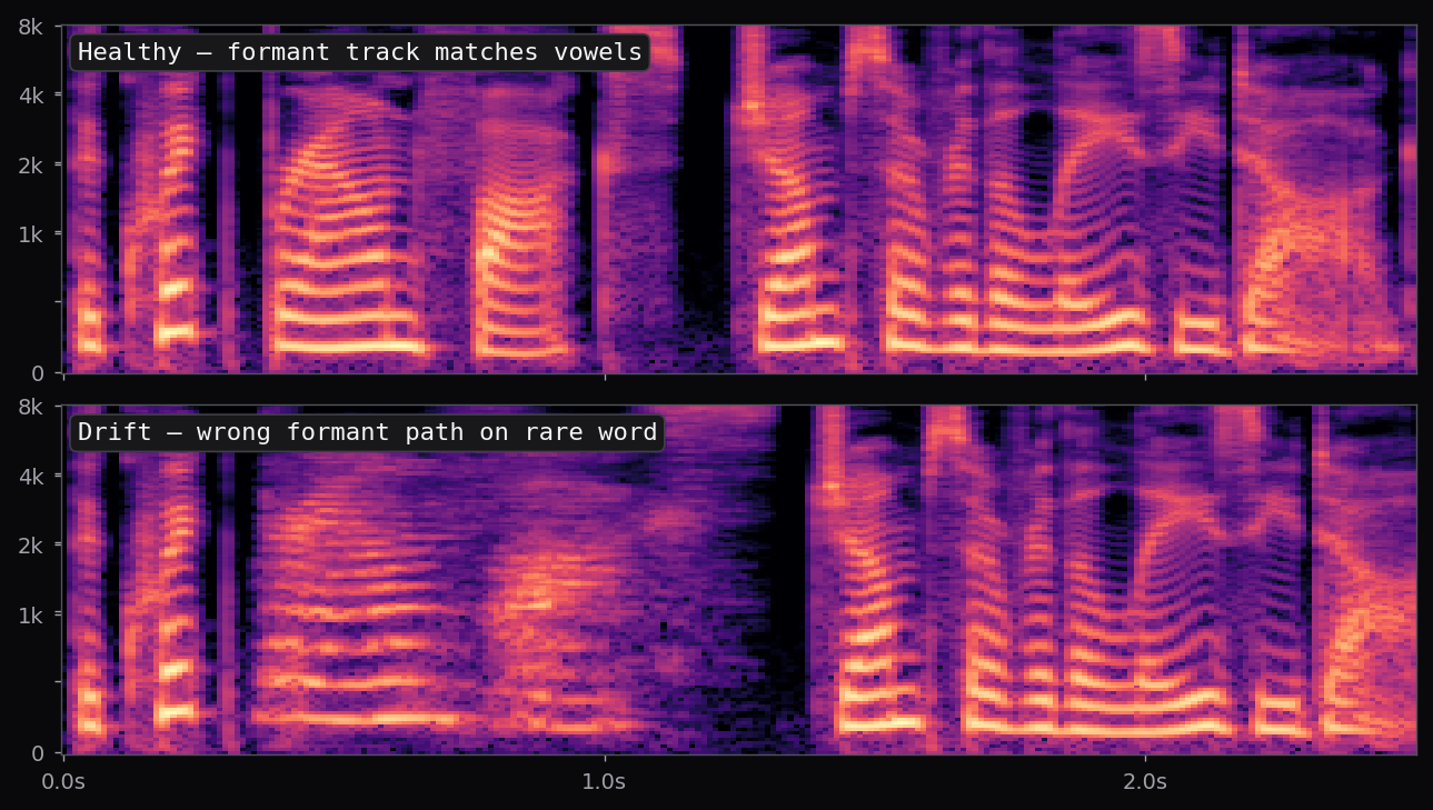
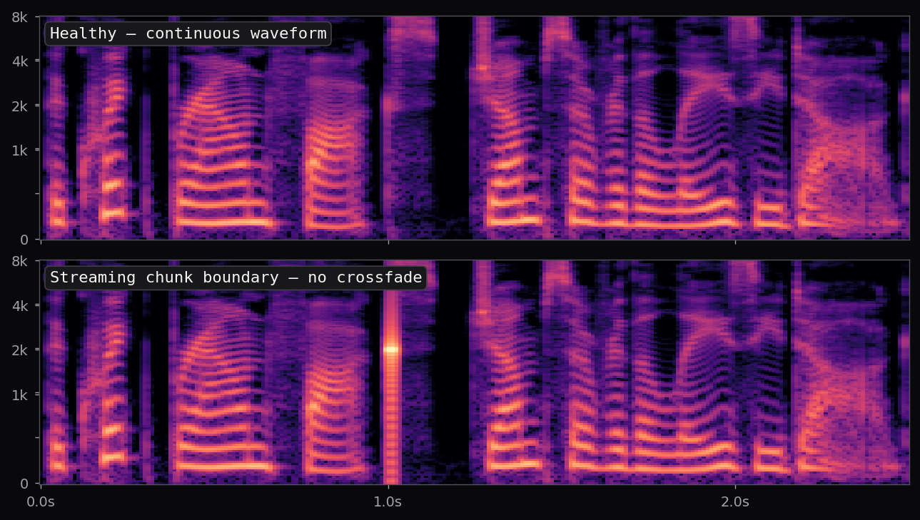
The af_heart, am_michael, and nine other voices used in the voice library above all ship with the stock Kokoro release. Apache 2.0 license. 54 voice packs at the time of writing, covering American, British, Japanese, Chinese, Spanish, French, Hindi, Italian, Portuguese. The spectrograms in this page's pipeline are rendered from audio that Kokoro generated locally, no API calls.

This is the end of the timeline, for now. The next entries will be the ElevenLabs and OpenAI comparison samples once their keys are wired in. The interesting thing is what the last 85 years have repeatedly shown: every representation introduced here — filter bank, spectrogram, LPC, formants, diphones, HMM parameters, mel-via-attention, dilated convolution audio, flow-matched codec tokens — is still visible somewhere in the pipeline on this page. The ladder is shorter than it looks.